Halo

A magic place for coding

0%

逻辑回归--LogisticRegression

Intro

  Logistic Regression,逻辑回归,实质上解决的是一个分类问题(我们之前说过,机器学习主要解决两类问题:回归和分类)。那为什么它又叫Regression呢?这是因为它用到了一个非线性函数——sigmoid函数,它给出的结果是一个概率值,而不是一个用于直接确定分类的离散值。下面我们就来仔细看看这个非常常用的分类算法。


原理

  首先我们还是基于传统的线性回归(Linear Regression)去思考一个分类问题,假设我们的模型预测值是$h_\theta(x)$,这个值的范围是不确定的,我们很难去找到一个不错的阈值去划分两类(因为模型的输出会受数据分布的影响,0.5并不是一个很科学的阈值)。这个时候我们就需要将$h_\theta(x)$的值压缩到一个相对小的区间中,最理想的情况就是压缩到[0,1]中,这样输出的就可以是一个概率了。

  幸运的是,我们能找到这样的函数——Sigmoid function(Logistic function)。它的曲线是这样的:

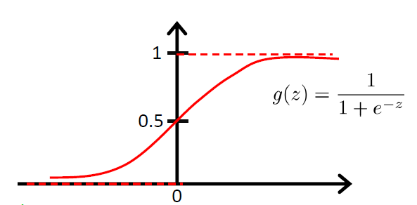
  从sigmoid的图像中我们可以看到一些我们想要的特性:

  • 当$z\rightarrow\infty$时,$g(z)\rightarrow1$;当$z\rightarrow -\infty$时,$g(z)\rightarrow 0$

  • $g(z)$的值被限制在了[0, 1]

  • sigmoid是光滑的,他的导数也是很容易求得:
    $$
    \begin{aligned}
    g^{‘}(x) &= \frac{d}{dz}\frac{1}{1+e^{-z}} \
    &=\frac{1}{(1+e^{-z})^2}(e^{-z}) \
    &= \frac{1}{(1+e^{-z})} \cdot(1 - \frac{1}{(1+e^{-z})}) \
    &= g(z)(1-g(z))
    \end{aligned}
    $$

  于是模型的输出就变为:
$$
h_\theta(x)=g(\theta^Tx)=\frac{1}{1+e^{-\theta^Tx}}
$$
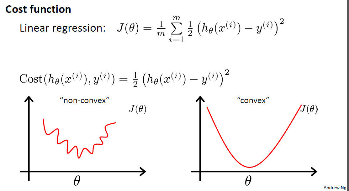
  建立好模型后,我们的工作就是需要找到这个最佳的$\theta$。之前我们用的是LMS,但是这里使用LMS得到的并不是一个凸函数,我们需要换另一种方式——最大似然法。

  最大似然法的思路是:我已经知道了若干个测试结果,我需要找出一组参数$\theta$,使得它们能够很好地模拟出这些测试结果。将每一个模拟的概率乘起来,极大化这个概率,我们就能得到最好的$\theta$。下面我们就来表示这些概率。

  首先我们假设:
$$
\begin{aligned}
&P(y=1|x;\theta)=h_\theta(x) \
&P(y=0|x;\theta)=1-h_\theta(x)
\end{aligned}
$$
  从条件概率的角度看,这两条式子的意思是:对于给定的$x$和$\theta$,模型的输出就是$x$属于类别1的概率。这个可以看作一个二项分布问题,所以我们可以将两条式子合并到一起:
$$
p(y|x;\theta)=(h_\theta(x))^y(1-h_\theta(x))^{1-y}
$$
  假设$m$个训练样本都是相互独立的,我们可以应用最大似然估计:
$$
\begin{aligned}
L(\theta) &= p(\hat{y}|X;\theta) \
&= \prod_{i=1}^mp(y^{(i)}|x^{(i)};\theta) \
&= \prod_{i=1}^m(h_\theta(x^{(i)}))^{y^{(i)}}(1-h_\theta(x^{(i)}))^{1-y^{(i)}}
\end{aligned}
$$
  一般来说,我们都不会直接极大化$L(\theta)$,而是极大化它的对数:
$$
\begin{aligned}
l(\theta) &= logL(\theta) \
&= \sum_{i=1}^my^{(i)}logh(x^{(i)}) + (1-y^{(i)})log(1-h(x^{(i)}))
\end{aligned}
$$
  极大化$l(\theta)$对我们来说就不是一件困难的事了,我们可以简单地使用GA(Gradient Ascend)。(特别注意,因为这里是要极大值,所以使用的Gradient Ascend)。推导过程如下:
$$
\begin{aligned}
\frac{\partial}{\partial\theta_j}l(\theta) &= (y\frac{1}{g(\theta^Tx)} -(1-y)\frac{1}{1-g(\theta^Tx)})\frac{\partial}{\partial\theta_j}g(\theta^Tx) \
&= (y\frac{1}{g(\theta^Tx)} -(1-y)\frac{1}{1-g(\theta^Tx)})g(\theta^Tx)(1-g(\theta^Tx))\frac{\partial}{\partial\theta_j}\theta^Tx \
&= (y(1-g(\theta^Tx))-(1-y)g(\theta^Tx))x_j \
&= (y-h_\theta(x))x_j
\end{aligned}
$$
  因此,最后的更新规则为:
$$
\theta_j := \theta_j+\alpha(y^{(i)} - h_\theta(x^{(i)}))x_j^{(i)}
$$
  有没有发现很眼熟?这个更新规则和LMS的更新规则是一样的!但是两者从本质上是不同的,这里的$h_\theta(x^{(i)})$是sigmoid函数。

  至此,Logistic Regression的原理推导就完成了!大家最好能够自己手动推导一次。

实战

  这里我用逻辑回归来预测疝气病马的存活问题。数据集来自UCI:传送门

数据预处理

  之前的博客给过处理UCI数据的一些代码模板,需要特别注意,这次的数据存在许多缺漏,因此我们需要手动处理一下。

  这里也简单地介绍一下如何处理缺失数据。处理缺失数据是特征工程一个很重要的部分,因为随便填补或删除会使得数据有可能加入了人为的噪声,所以我们需要有多种方法去填补。以下是几个典型的方法:

  • 使用可用特征的均值(或众数)来填补缺失值;
  • 使用特殊值来填补缺失值,如-1(相当于添加了一个新的类别)
  • 直接忽略掉有缺失值的样本(对于缺失属性较多的样本可以这样做)
  • 使用相似样本的均值填补缺失值
  • 使用其他机器学习的方法预测缺失值(如使用随机森林来预测,相当于根据已知特征来预测缺失的特征)

  对于这个样本,我的处理主要有两个:

  • 使用0来填补缺失值,因为0对回归系数不会有影响,不会添加人为的bias。
  • 如果某个样例的标签(label)缺失,则直接丢弃这个样例。(相当于不知道答案就不用做题)
1
2
3
4
5
6
7
8
9
10
11
12
13
14
15
16
17
18
19
20
21
22
23
24
25
26
27
28
29
30
31
32
33
34
35
36
37
38
39
40
41
42
43
44
import numpy as np

frTrain = open('./horse_colic_data.txt')#训练数据
frTest = open('./horse_colic_test.txt')#测试数据
trainSet=[]
for line in frTrain.readlines():
currLine=line.strip().replace('?', '0').split('\t')
temp = currLine[0].split(' ')
lineArr=[]

for i in range(22):
if i == 2:
continue
else:
lineArr.append(float(temp[i]))
if (temp[22] == '1'):
lineArr.append(1)
else:
lineArr.append(0)
#print(lineArr)
trainSet.append(lineArr)
trainSet.pop(132)
print(type(trainSet))
np.savetxt('processedHorseColicTraining.txt', trainSet, fmt='%.6f', delimiter='\t')

testSet = []
for line in frTest.readlines():
currLine=line.strip().replace('?', '0').split('\t')
temp = currLine[0].split(' ')
lineArr=[]

for i in range(22):
if i == 2:
continue
else:
lineArr.append(float(temp[i]))
#print(type(temp[22]))
if (temp[22] == '1'):
lineArr.append(1)
else:
lineArr.append(0)
#print(len(lineArr))
testSet.append(lineArr)
np.savetxt('processedHorseColicTest.txt', testSet, fmt='%.6f', delimiter='\t')

构建Logistic回归分类器

  定义sigmoid函数,使用梯度上升法求解。

1
2
3
4
5
6
7
8
9
10
11
12
13
14
15
16
17
18
19
20
21
22
23
24
25
26
27
28
29
30
from numpy import *
import pandas as pd
import numpy as np
def loadDataSet():
file = './processedHorseColicTraining.txt'
df = np.loadtxt(file)
dataMat = df[:, 0:-1]
#dataMat = np.insert(dataMat, 0, 1, axis=1)
labelMat = df[:, -1]
return dataMat, labelMat

dataMat, labelMat = loadDataSet()
print(dataMat.shape)

def sigmoid(x):
return 1/(1+exp(-x))

def gradientAscent(dataMatIn, classLabels):
m,n=shape(dataMatIn)
print(n)
classLabels = np.array([classLabels]).T
weights = np.ones((n,1))
alpha = 0.001
max_iter = 500

for _ in range(max_iter):
h = sigmoid(np.dot(dataMatIn, weights))
error = classLabels - h
weights += alpha * np.dot(dataMatIn.T,error)
return weights

随机梯度上升法

  这里试用随机梯度上升法,每次梯度更新仅用到了一个样例。

1
2
3
4
5
6
7
8
9
def stochasticGradientAscent(dataMatIn, classLabels):
m, n = np.shape(dataMatIn)
alpha = 0.01
weights = np.ones(n)
for idx in range(m):
h = sigmoid(sum(dataMatIn[idx] * weights))
error = classLabels[idx] - h
weights += alpha * error * dataMatIn[idx]
return weights

构建输出部分

  前面提到,Logistic Regression的输出是一个概率值,我们需要将这个概率值转化为一个类别,用0.5作为阈值是一个不错的选择。

1
2
3
4
5
6
def classifyVector(inX, trainWeights):
prob = sigmoid(sum(np.dot(inX,trainWeights)))
if prob > 0.5:
return 1
else:
return 0

测试

  使用测试集来评估模型的效果。同时还可以对比两种不同的梯度上升法

1
2
3
4
5
6
7
8
9
10
11
12
13
14
15
16
17
18
19
20
21
22
23
24
25
26
test_file = './processedHorseColicTest.txt'
df_test = np.loadtxt(test_file)
testDataMat = df_test[:, 0:-1]
testLabelMat = df_test[:, -1]
print(testDataMat)


import time
start = time.clock()

result2 = advancedStochasticGradientAscent(dataMat, labelMat, 500)

end = time.clock()
print (end - start)

errorCount = 0;numTestVec = 0;
[rows, cols] = testDataMat.shape

for i in range(rows):
numTestVec += 1
if classifyVector(array(testDataMat[i, :]), result2) != int(testLabelMat[i]):
errorCount += 1

print(errorCount, numTestVec)
errorRate = (float(errorCount) / numTestVec)
print('the error rate of this test is: %f' % errorRate)

  测试结果:

  • 随机梯度上升法,错误率约37%

  • 常规的梯度上升法,错误率约29%

    考虑到整个数据集的缺失率在30%左右,这个错误率也是可以接受的范围了。

使用Sklearn

  使用Sklearn构建LogisticRegression模型非常简单,只需要定义几个变量就可以了。

1
2
3
4
5
6
7
8
9
10
11
12
13
14
15
16
17
18
19
20
21
22
from sklearn.linear_model import LogisticRegression
import numpy as np

def colicSKlearn():
file = './processedHorseColicTraining.txt'
df = np.loadtxt(file)
dataMat = df[:, 0:-1]
labelMat = df[:, -1]

test_file = './processedHorseColicTest.txt'
df_test = np.loadtxt(test_file)
testDataMat = df_test[:, 0:-1]
testLabelMat = df_test[:, -1]

classifier1 = LogisticRegression(solver='liblinear', max_iter=20).fit(dataMat, labelMat)
classifier2 = LogisticRegression(solver='sag', max_iter=5000).fit(dataMat, labelMat)

test_accuracy = classifier1.score(testDataMat, testLabelMat) * 100
print('Accuracy: %f%%' % test_accuracy)

if __name__ == '__main__':
colicSKlearn()

  这里简单解释一下模型的参数:

  • solver:优化算法。选项为:
    • liblinear:坐标下降法
    • lbfgs:拟牛顿法,使用二阶导数来优化(海森矩阵)。
    • newton-cg:牛顿法的一种。
    • sag:随机平均梯度下降
    • saga:SAG的加速版本

  测试的结果正确率为73.529412%,似乎比我们自己写的要好一点点。


总结

  Logistic Regression是机器学习中分类算法的基础,应用的范围非常广,实际效果也非常不错。一定要注意区分它和线性回归,它的数学原理推导部分是重点!至于实际应用,调用sklearn的模型就可以了。

Welcome to my other publishing channels