Intro
决策树是一类常见的机器学习方法,它解决的是分类问题。以二分类任务为例,我们实质上是对每个样本做出这样的提问:“这个样本属于正样本吗?”。模型的回答就是我们对于这个问题的决策。决策树是基于树结构的决策方法,它的形式就是对于一个样本进行一系列的提问与判断,最终做出决策。
在Tom Mitchell的《Machine Learning》中,对决策树的描述是这样的:
Decision tree classify instances by sorting them down the tree from the root to some leaf node, which provides the classification of the instance
原理
决策树的构成
决策树是以树结构为基础的,一般包含:
- 一个根结点(root node)
- 若干个内部结点(node)
- 若干个叶子结点(leaf node)
从整棵树的角度来看,决策树又可以看成是以下两部分构成的:
- Node:A test of some attribute of the instance(节点是对一个属性的测试)
- Branch:One of the possible values for this attributes(边是一个属性的可能取值)
看下面的例子来理解:
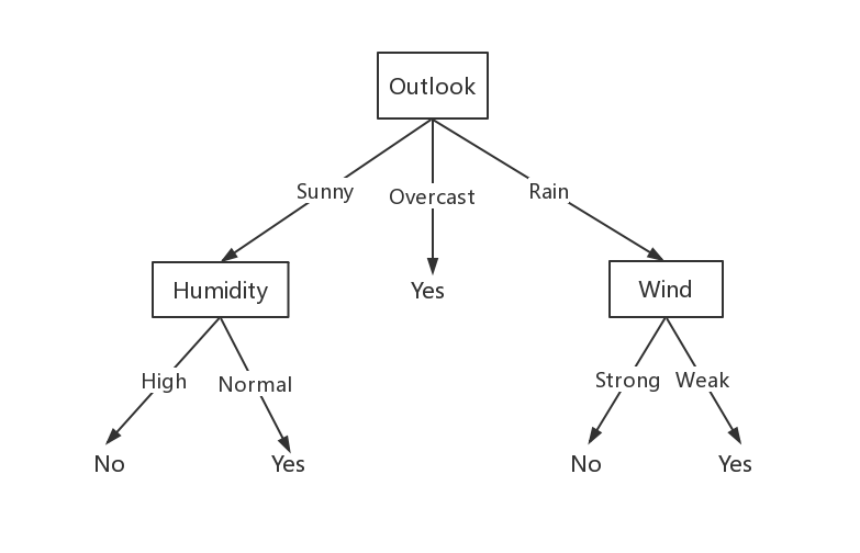
上面的例子中,Outlook是根结点,Humidity、Wind是内部结点,Yes和No是叶子节点。以Outlook为例,该属性的取值有三个:Sunny、Overcast、Rain,分别对应三条边。
从另一个角度来看,其实决策树表示的是析取范式(A disjuction of conjunctions)。将上述例子转化为析取范式:
$$
(Outlook = Sunny \wedge Humidity=Normal) \
\vee (Outlook = Overcast) \
\vee (Outlook=Rain \wedge Wind=Weak)
$$
划分选择
决策树的原理很符合我们日常的思维方式,理解起来并不难,但是难点在于如何去合理地构建一颗泛化能力强的决策树——即如何选择使用哪个属性去做测试?
我们的目的是:随着划分的不断进行,决策树分支结点所包含的样本应该尽可能地属于同一类。如果分支节点的样本都是属于同一类的,那么这个就是叶子结点了,也就是完成了决策判断了。所以这样一个决策的过程是向着结点纯度(purity)高的方向进行的。
信息熵(Entropy)
信息熵(Entropy)是用于描述信息的纯度,它是信息论的一个概念。应用在我们的分类问题中,它可以理解为:
It characterizes the impurity of an arbitray collection of examples.
直接来看公式理解(假设样本集为S,S只有一个属性,将所有样本划分为正样本和负样本):
$$
Entropy(S)=-p_{\oplus}\log_{2}p_{\oplus} - p_{\circleddash}\log_{2}p_{\circleddash}
$$
其中,符号的定义是:
- $p_{\oplus}$:The proportion of positive examples in S
- $p_{\circleddash}$:The proportion of negative examples in S
- 定义:$log_20 = 0$
举例说明一下,令$S=14$,正样本为9,负样本为5,则:
$$
Entropy([9+,5-])=-\frac{9}{14}log_2\frac{9}{14} - \frac{5}{14}log_2\frac{5}{14} = 0.940
$$
然后我们来解读一下这个信息熵实际的意义是什么?

如图我们可以看到,当正样本占比为0或1时,样本中只有一类样本,此时entropy为0,即S不混乱;当正样本占比0.5时,样本中正负样本数量相当,此时entropy为1,即S中非常混乱。
对于entropy,Tom Mitchell给出的另一种解读是:
It specifies the minimum number of bits of information needed to encode the classification of an arbitrary member of S
对S中任意一个成员编码所需要的最小数量的bit。
当然,实际问题中,每一个属性不一定只有两种取值,这时候公式变形为:
$$
Entropy(S) = \sum^C_{i=1}-p_ilog_2p_i
$$
$p_i$ is the proportion of $S$ belonging to class $i$。
信息增益(Information Gain)
前面提到,我们希望的划分是能够提升减少信息熵的,信息增益就是用于衡量划分前后信息纯度的提升的量。也就是说,信息增益越大,该划分导致的信息纯度提升越多,我们就认为这个划分越好。
信息增益的计算公式如下:
$$
Gain(D, a) = Entropy(D) - \sum_{v\in Value(A)}\frac{|S_v|}{S}Entropy(S_v)
$$
其中$Value(A)$是属性$A$所有可能取值的集合。$S_v={s\in S|A(s) = v}$。
怎么理解信息增益这条公式呢?前面提到这是计算划分前后信息熵的变化,那么划分前的信息熵就是$Entropy(D)$,划分后的则是一个期望——每个子划分的entropy的和求平均,权重由样本占比决定。
Tom Mitchell也给出了对于信息增益的另一种解释:
The value of Gain(S, A) is the number of bits saved when encoding the target value of an arbitrary member of S, by knowing the value of attribute A.
信息增益是当知道属性A的取值后,对该样本集S编码所需要的bits数量的减少。
举例说明一下,已知:
$$
\begin{align}
Values(Wind) &= Weak, Strong \\
S&=[9+,5-] \\
S_{Weak} &= [6+, 2-] \\
S_{Strong} &= [3+, 3-]
\end{align}
$$
计算Information Gain,得到:
$$
\begin{align}
Gain(S, Wind) &= Entropy(S) - \sum_{v\in {Weak, Strong}}\frac{|S_v|}{S}Entropy(S_v) \\
&= Entropy(S) - \frac{8}{14}Entropy(S_{Weak}) - \frac{6}{14}Entropy(S_{Strong}) \\
&= 0.940 - \frac{8}{14} \times 0.811 - \frac{6}{14} \times 1.00 \\
&= 0.048
\end{align}
$$
增益率(Gain Ratio)
这一部分是对信息增益的改进,初学者可以跳过这一部分的阅读,不影响后续的内容。
在构建机器学习的模型中,我们的模型不能有太强的bias,过强的bias会导致模型很容易偏向一部分数据,从而导致过拟合现象,减弱模型的泛化能力。使用Information Gain就存在这个问题。Information Gain偏向的是那些有多个取值的属性,但实际上这种bias是不好的。
为什么呢?因为类别过多的话,说明我们分类的很细,分出来的子类可能包含的个数就很小,而他们的类别很可能都是一样的,因此他们的纯度就会很高。例如,我们使用索引来进行分类,每个子类都将只包含一个样例,每个子类的entropy都会是0,根据Information Gain,这种分类是最优的,但实质上这样的划分并不具有任何意义。
为了减少这种natural bias,我们可以采用Gain Ratio来代替Information Gain。来看看Gain Ratio的计算公式:
$$
SplitInformation(S, A) = -\sum^c_{i=1}\frac{|S_i|}{|S|}log_2\frac{|S_i|}{|S|} \
GainRatio(S, A)=\frac{Gain(S, A)}{SplitInformation(S, A)}
$$
从上面看出,Gain Ration比Gain多了一个分母SpliteInformation,这个SplitInformation反映了属性$A$的取值多少。如果$A$取值很多,那么这个值就会很大(因为log一个接近于0的数是一个绝对值很大的数)。也就是说,The SplitInformation(S, A) term discourages the selection of attributes with many uniformly distributed values。这样就达到我们的目的了。
基尼指数(Gini Index)
这一部分是关于CART的内容,初学者可以跳过这一部分,不影响后续的阅读。
选择划分特征,除了可以使用上面提到的Information Gain、Gain Ratio,还有这里要提到的Gini Index。注意,这里用的是基尼指数(Gini Index),而不是基尼系数(Gini Coefficent)!它同样表示的是信息的纯度。看看它的计算公式:
$$
\begin{align}
GiniIndex(D) &= \sum_{k=1}\sum_{k^{‘}\neq k}p_kp_{k^{‘}} \\
&= 1 - \sum_{k=1}p_k^2
\end{align}
$$
通俗地说,基尼指数反映了从数据集$D$中随机抽取两个样本,其类别不一样的概率。所以基尼指数越小,数据集$D$的纯度越高。
我们定义数据集$D$中属性$a$的基尼指数为:
$$
GiniIndex(D, a) = \sum^V_{v=1}\frac{|D^v|}{D}Gini(D^v)
$$
然后我们选择基尼指数最小的属性作为最优的划分属性。
实战
实战分类两部分,第一部分使用简单的数据手动构建一个决策树;第二部分使用sklearn库来构建决策树。
放贷预测
这个案例中,我们简单地模拟一个放贷预测模型。假设我们统计的数据如下:
- 年龄:0表示20-30岁,1表示30-60岁,2表示60岁及以上;
- 是否有工作:0表示没有工作,1表示有工作;
- 是否有房子:0表示没有房子,1表示有房子;
- 信贷情况:0表示不好,1表示好,2表示非常好
- 【标签值】是否给予贷款:
yes代表给予贷款,no代表不给予贷款。
构建数据集
数据量非常小,直接手动输入到代码中。
1 | def createDataset(): |
计算Entropy
计算Gain的时候需要用到Entropy,因此把计算某个数据集的Entropy单独写成函数。根据上面的公式编写就可以了。
1 | def calculateEntropy(dataset): |
划分子集
在计算Gain时需要模拟划分出来的许多子集,在确定划分属性后需要真正的划分出子集,因此将反复调用的功能单独成一个模块。
1 | def splitDataset(dataset, axis, value): |
选择最优划分属性
通过对当前数据集计算每一个属性的Gain,选择Gain最大的一个属性作为划分属性。
1 | def chooseBestFeatureToSplit(dataset): |
构建决策树模型
递归构建决策树,根据输入的当前数据集、属性值列表和已划分属性列表,寻找当前最优的划分属性进行划分,将划分后的数据集、属性值列表、已划分属性列表递归构建子树。
1 | ''' |
countMajority(classlist)返回的是出现次数最多的标签值,当决策树构建完后返回。
1 | def countMajority(classlist): |
运行
1 | if __name__ == '__main__': |
运行结果:
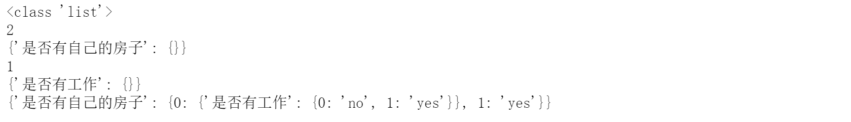
我们可以看到构建的树以字典的形式存储下来了。注意这里我们只看到了两个属性:是否有自己的房子、是否有工作,而没有其他的属性。这是因为只依靠这两个属性就能把数据集划分,所以就不需要更多的属性了。
可视化
我们希望用plt库来将决策树可视化。这一部分不是重点,因此不详细介绍。
1 | # 决策树可视化 |
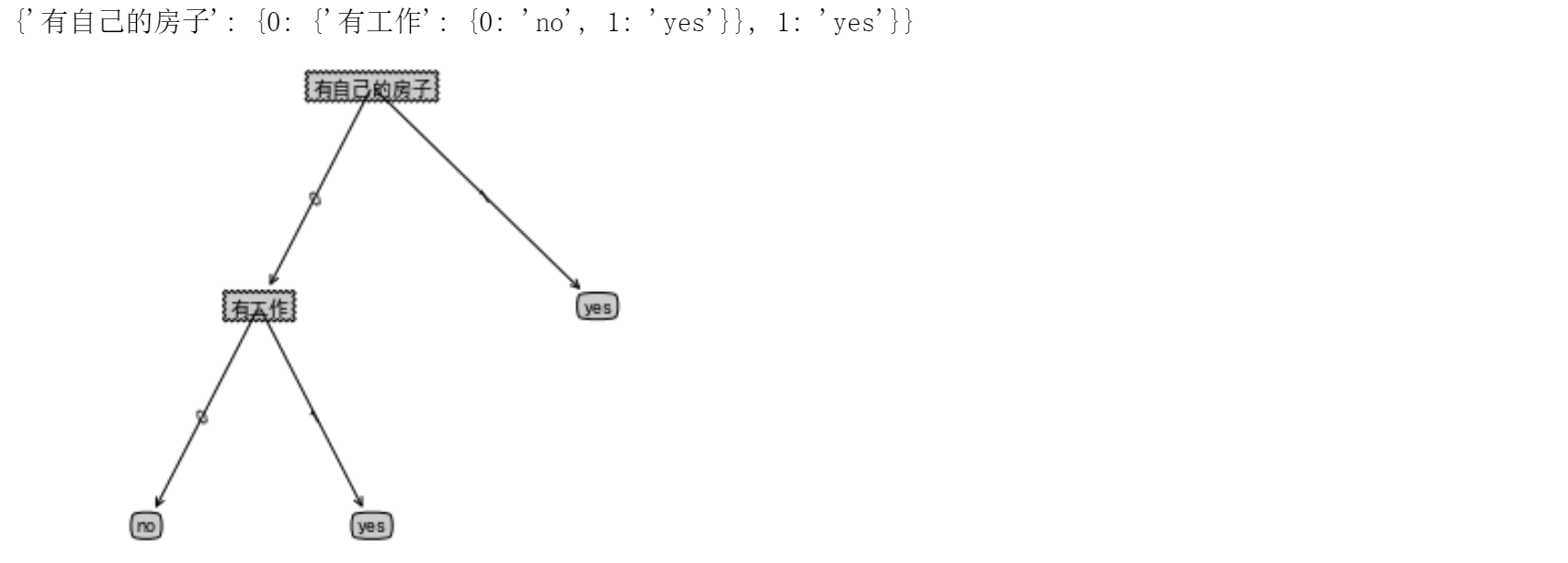
运行结果:
测试
我们简单测试一下决策树的效果。简单构建一个测例[0,1]。
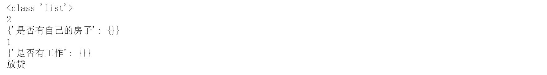
预测结果是同意放贷。
存储决策树
由于我们自己建立的决策树是一个字典,所以我们可以将它转变为字符串的形式存储为一个txt文件,之后使用的时候就不需要重新构建,直接预测即可。
1 | # 存储决策树 |
隐形眼镜预测
这里我们使用决策树预近视者需要佩戴何种隐形眼镜。所用数据集是UCI提供的 Lens Date Set:http://archive.ics.uci.edu/ml/datasets/Lenses
数据准备
这个数据集非常小,只有24个样例,而且是完成且无噪声的,非常适合构建模型。
每个样例包含4个属性和1个标签值:
- Age of the patient(患者年龄): (1) young, (2) pre-presbyopic, (3) presbyopic
- Spectacle prescription(视力诊断): (1) myope(近视), (2) hypermetrope(远视)
- Astigmatic(散光): (1) no, (2) yes
- Tear production rate(泪流率): (1) reduced(偏少的) (2) normal
- 【label】 Class:(1) Hard lens; (2) Soft lens; (3) No lens
因为数据非常干净,所以数据准备只需要读入,切分成特征部分和标签值部分即可。
1 | import numpy as np |
构建决策树
这里我们尝试使用sklearn库提供的决策树来进行构建。官方文档:https://scikit-learn.org/stable/modules/tree.html。这里的决策树默认使用基尼指数来作为划分的评判标准。
1 | from sklearn import tree |
测试
随机构造一个样本进行预测。
1 | res = clf.predict([[2,1,1,1]]) |
决策树可视化
对于上面测试的样本,你无法确定是否正确,我们可以通过可视化决策树来分析整个决策过程。这里需要用到Graphviz。
先安装pydotplus,命令行输入:
1 | pip3 install pydotplus |
再安装Graphviz,配置环境变量:
- 下载地址:https://graphviz.gitlab.io/_pages/Download/Download_windows.html。
- 安装教程:https://blog.csdn.net/Candy_GL/article/details/79684947
安装后,确定labels,然后可以直接将构建好的决策树模型使用graphviz来可视化为pdf。
1 | from sklearn.externals.six import StringIO |
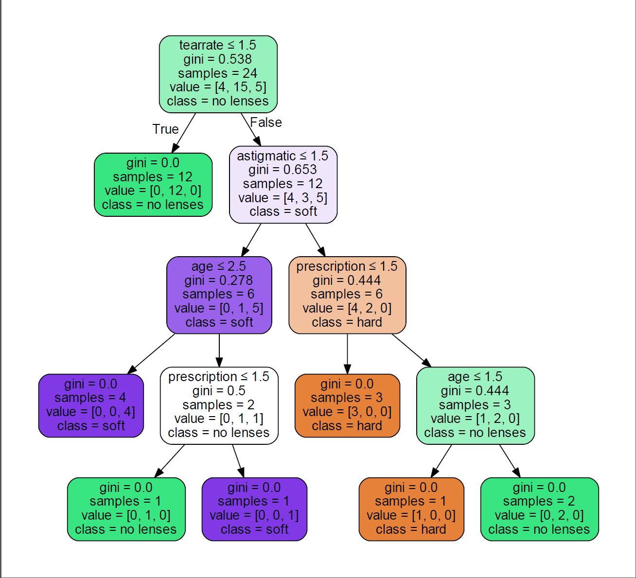
可以看到这里的决策树使用的上面提到的Gini Index来作为划分标准的,它将离散型的数值看成连续性数值来处理(回归树)。每个节点标出了以下信息:
- gini(对应的基尼指数):该结点数据集的基尼指数;
- samples(包含的样本数量):该结点数据集的大小;
- 分类标准(如根节点的tearrate$\le$1.5):该结点是按什么分类的;
- value(每个类别对应的样本数量):该结点数据集每个类别所包含的样本数量;
- class(包含最多的类别):该结点数据集样本中出现最多的类。
以上就是sklearn库中决策树的一些使用了,非常简便。
总结
至此我就讲关于决策树的一些基本知识分享给大家了。通过两个简单的实战,分别自己实现了决策树和使用了sklearn的决策树,并对决策树做了可视化处理,相信这样能够更好地理解决策树的工作原理。如果本文中有什么不对的地方,欢迎提出宝贵的意见!谢谢您的支持!

