Intro
最小均方法,Least Mean Square(简称LMS),是一种通过最小化误差的机器学习算法。它是机器学习常用的算法之一,通常结合梯度下降法来求解出最优的参数。
LMS算法
loss function
所谓均方,就是误差的平方的均值。LMS训练法则,可以简述为以下式子,通常也叫做代价函数(cost function):
$$
J(w)=\frac12\sum^m_{i=1}{h(x^{(i)})-y^{(i)}}^2
$$
其中,$h(x^{(i)})$为学习网络的输出信号,$y^{(i)}$为导师信号。
Gradient Descent
我们的目的就是要通过某种方法,来最小化这个代价函数。通常使用的方法是梯度下降法(gradient descent),因为对于凸优化问题而言,导数值为0的地方就是全局极小值。所以我们可以利用梯度来指引我们向极小值处走近。
梯度下降法的更新规则为:
$$
\theta_j := \theta_j - \alpha\frac{\partial}{\partial\theta_j}J(\theta)
$$
**注意:**这里的$\theta_j$的更新是同步的(即是用相同的$J(\theta)$),也就是说,更新完所有的$\theta_j(j=0,\dots,n)$后,才算下一个梯度。
然后我们推导梯度的计算:
$$
\begin{aligned}
\frac{\partial}{\partial\theta_j}J(\theta) &= \frac{\partial}{\partial\theta_j}\frac{1}{2}(h_\theta(x) - y)^2 \
&=2 \cdot \frac{1}{2}(h_\theta(x) - y) \cdot \frac{\partial}{\partial\theta_j}(h_\theta(x) - y)
\
&=(h_\theta(x) - y) \cdot\frac{\partial}{\partial\theta_j}(\sum^n_{i=0}\theta_ix_i-y) \
&=(h_\theta(x)-y)x_j
\end{aligned}
$$
因此对于某一个样例来说,其更新规则为:
$$
\theta_j:=\theta_j+\alpha(y^{(i)}-h_\theta(x^{(i)}))x_j^{(i)}
$$
可以看出,当预测值$h_\theta(x^{(i)})$和真实值$y^{(i)}$相等时,该参数并不会更新;而当它们不相等时,参数会按照他们的difference来更新参数,这样从直观上来说也是合理的。
梯度下降法给我们提供了一种求代价函数极小值的方法,它有很多变种,下面就介绍几种常用的方法。特别注意,仅当我们面对的是一个凸优化问题,梯度下降法才能够保证让我们找到全局最优解。
Batch Gradient Descent
批梯度下降法,其本质是每一轮迭代使用整个训练集去更新权重,即考虑了整体样本的梯度。其算法伪代码为:
$Repeat ;Until ;convergence; {$
$ \quad \theta_j:=\theta_j+\alpha\sum^m_{i=1}(y^{(i)} - h_\theta(x^{(i)}))x_j^{(i)};;(for ; every; j)$
$}$
Stochastic Gradient Descent
随机梯度下降法,其本质是每次迭代只用一个样例去计算梯度,更新参数。相比起批梯度下降法,随机梯度下降法大大提高了计算效率。从理论上说,SGD能让我们更快地找到最佳的参数,但是它有可能无法收敛到极小值,而是在极小值附近波动。但实际情况时,对于极小值附近的值也是对极小值的一个很好的近似,因此在数据集较大的情况下,SGD的实际效果是优于BGD的。其算法伪代码为:
$Loop ; {$
$ \quad for ;i=1 ;to;m, ; {$
$ \quad \quad \theta_j:=\theta_j+\alpha(y^{(i)} - h_\theta(x^{(i)}))x_j^{(i)};;(for ; every; j)$
$ \quad }$
$ } $
实例
我们以拟合一条直线作为例子,以下给出一些前提定义:
- 训练样例$X_i(a_i, b_i)$,$i = 1,2,…,n$,$n$为样本大小
- 导师信号$D=[d_1, d_1,…,d_i]$,$i = 1,2,…,n$,$n
$为样本大小 - $h(X_i)$是在假设$h$下预测得到的预测值
- 权值矩阵$W=[w_0,w_1]$
- 目标函数$w_0x+w_1y$
- 学习率(步长)$\eta$4,$0\lt \eta \lt 1$
- 更新法则:$W(n+1) = W(n) + \eta * X_i * (d_i - h(X_i))$
我们输入的数据是一系列的点,以及导师信号D(target value)。我们期望的输出是描述这个直线的权值矩阵$W=[w_0,w_1]$。
初始化变量
初始化一些变量,其含义注释有描述。
1 | import numpy as np |
激活函数
激活函数(Activation Function)可以视为一个神经元对输入的反馈。举个简单的例子来帮助大家理解,我们听到一个消息,可能会激动,也可能不会激动。这个激活函数就是来判断我们是否会激动的函数。具体看,假如我们得知的是考试分数,80分以下我们就不会激动,80分以上我们就激动,那么这个激活函数就可以写为:
1 | def sgn(x): |
那么在我们这个例子中,我们要确定一条直线,那么我们给出的是这个点在线的上方(1)还是下方(0)。
1 | # Activation Function |
输出信号
在每一个神经元我们要输出预测值,这是根据上面给出的激活函数得出的。
1 | def get_v(W, x): |
dot是矩阵乘法,W.T是代表W的转置。因此np.dot(W.T, x))是一个实数。
计算误差
误差是预测值与导师信号之差。
1 | def get_error(W, x, d): |
更新权重
按照上面给出的权重更新公式来计算更新后的权重。
1 | # Update Weights |
返回一个pair,第一部分是更新后的参数,用于赋值给W,第二部分是当前这个样本$X_i$的误差,用来计算均方。
训练过程
1 | # Training |
这里的训练过程我们称为批量的,因为每一个循环都对所有的样本进行训练,然后调整权重。这种做法开销比较大,但是精度较高。
测试部分
我们先对训练数据进行测试,然后再对两个单独的例子进行测试。
1 | # Test |
完整代码
1 | ''' |
分析
先给出程序运行结果: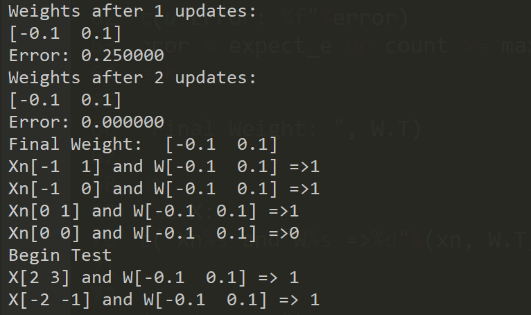
可以看出,实际上我们训练出来的直线是y=x。从拟合的角度看,我们根据给出的一系列点,最后拟合出一条直线。从分类的角度看,这条直线将二维平面分成两部分,在直线上方的标记为1,在直线下方的标记为0。
在这个例子中,训练两次后就已经满足了我们期望的误差,这是因为我给出的点是比较好的,很容易识别出来。对于其他的直线和数据集,可能需要多次的训练才能得到结果。
总结
LMS算法本质上是给我们提供了一种判断方法,判断当前的权值对于实际预测的准确性。机器学习的任务就是去极小化这个误差。先来看看这里用到的更新方法:$W(n+1) = W(n) + \eta * X_i * (d_i - h(X_i))$
我们这样理解:
- 当$(d_i - h(X_i))=0$时,权值不会改变。这说明当导师信号和我们预测的信号一致时,我们就认为当前的分类是正确的,无需做出改变。
- 当$(d_i - h(X_i))$为正时,说明预测值比导师信号要小,所以需要在原权值的基础上增加一定的比例。反之亦然。
- 当$X_i=0$时,权值不会改变。这说明当这个特征$X_i$没有出现时,它的权值是不会因为误差而改变的。
当然,在实际应用中,我们更多使用的是梯度下降法,这会在之后的博客中和大家分享,这里就只分析LMS算法。谢谢您的支持!

